How Project Rhino leverages Hadoop to build a graph of the music world

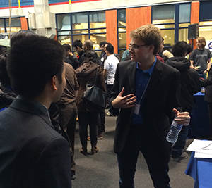
This last week Tony Dong, Omid Mortazavi, Vineet Nayak and I presented Project Rhino at this years ECE Capstone Design Symposium at the University of Waterloo.

Project Rhino is a music search engine that allows you to ask questions about the music world in plain English. Check out a demo video here.

We noticed there is a ton of data available about the music world but that they were disconnected. There was no easy way to explore the relationships in the music world.

This project allows a user to express an English query, that is then transformed into a traversal over the music data we have collected. All of the data was retrieved from freely available Creative Commons sources. However, integrating the data from disparate sources is non-trivial.

Here are some of the questions Project Rhino can answer:

• Find artists similar to "The Beatles" and played in "Waterloo, Ontario"
• Find artists from Canada and similar to "Vampire Weekend"
• Find songs by artists from Australia and similar to artists from Germany
• Show venues where artists born in 1970 and from Japan played

Aside from the complexities of data integration, the sheer volume of data (100+ GB of compressed JSON) makes this project challenging.

In this post I focus on one aspect of the ETL pipeline I developed for Project Rhino, the construction and insertion of the graph into our graph database.

The Graph Database

We used Titan on top of Cassandra to store our graph. It’s a pretty cool project and worth checking out. They provide a nice graph abstraction and excellent graph traversal language called Gremlin.

When we first came up with the idea for this project at Morty’s Pub, we were going to build our own distributed graph database from scratch. Titan saved us a lot of pain.

The people who produce Titan have a batch graph engine built on top of Hadoop called Faunus. It’s pretty cool but we didn’t end up using it for some of the reasons I’ll talk about later.

Rhino’s Batch Graph Build

The final and most intensive stage of the pipeline is graph construction. This is when the data is combined to create the graph. The graph is made up of two components: nodes with properties (ex. an artist) and edges between nodes with properties (ex. writtenBy). This stage outputs a list of graph nodes and then a list of graph edges. This process is managed by a series of Hadoop MapReduce jobs.

Hadoop Vertex Format

The first step is to transform the intermediate form tables into nodes and edges. Since Hadoop requires that data be serialized between steps, I needed a way to represent the graph on disk. I chose to use a Thrift Struct.

Here’s the Thrift definition for a vertex in the ETL pipeline:

struct TVertex {
  1: optional i64 rhinoId,
  2: optional i64 titanId,
  3: optional map<string, Item> properties,
  4: optional list<TEdge> outEdges
}

The rhinoId is the ID used in the intermediate tables. This is the ID we assigned as part of the ETL process. titanId refers to the identifier Titan generates for the vertex. The distinction is discussed in further detail in the Design Decisions section below.

The outEdges field is a list of graph edges with the current vertex as its source (or left hand of the arrow).

The properties field is a map of string keys to typed value as described here:

union Item {
  1: i16 short_value;
  2: i32 int_value;
  3: i64 long_value;
  4: double double_value;
  5: string string_value;
  6: binary bytes_value;
}

Here is the Thrift definition for an edge in the ETL pipeline.

struct TEdge {
    1: optional i64 leftRhinoId,
    2: optional i64 leftTitanId,
    3: optional i64 rightRhinoId,
    4: optional i64 rightTitanId,
    5: optional string label,
    6: optional map<string, Item> properties
}

MapReduce Jobs

Vertex Jobs

The first set of jobs is responsible for converting the intermediate tables into Thrift. Here is an example of the conversions of two tables into its Thrift form.

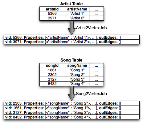
Now all of the tables follow the same structure and we can treat all vertices the same way!

Edge Jobs

The next set of jobs transforms intermediate edge tables into edges. In practice, vertex and edge conversion jobs can (and are) run simultaneously.

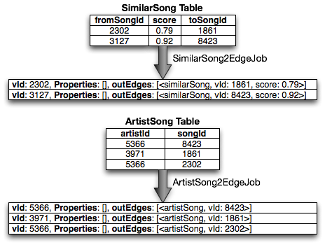
Note that instead of producing TEdge structures, TVertex structures are produced. To facilitate bulk loading, edges are treated like vertices that have no properties. This allows the next stage to treat records from vertex jobs and edge jobs identically.

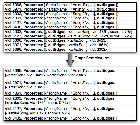
Graph Combine Job

The next stage is a single job that combines vertices and edges by joining them on titanVertexId. As pictured, both vertex and edge records are combined together so that each vertex appears only once in the output.

Vertex Insert Job

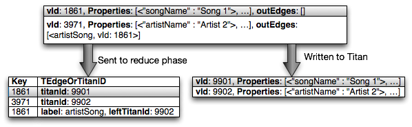
The Vertex Insert Job is the first job that actually inserts data into the graph. There are two important phases of this job, the mapper and the reducer. The mapper, as shown below writes each vertex to Titan.

When it writes the vertex to Titan, it receives an opaque ID that Titan has assigned to the vertex. The mapping between rhinoID and titanId is written out so that it can be used in the reduce phase to be matched with all possible incoming edges.

Next, all of the outgoing edges are written out, grouping by target instead of source vertex. The key is the target (the right hand vertex) rhinoID and the value now includes the source (the left hand vertex) titanId.

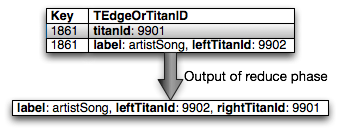
In the reduce phase, all of the records with the same rhinoId (including the record showing the mapping to Titan ID) are processed at the same time. The titanId for the given Rhino ID will always appear first due to the use of a custom sort function not described here.

For each subsequent record (now all edges), the rightTitanId is added to the edge and written out. At this point the edges could be written directly to Titan. I’ll talk about why we don’t later on.

Edge Insert Job

The edge insert job is fairly straightforward. The mapper reads in the edges one at a time and adds an edge between the source and target vertices. This is a map only job and there are no outputs other than the insertions into the graph.

Design Decisions

Custom Batch Framework

I initially tried to use Titan’s own batch framework. Two problems arose. First, there was limited room for insert optimizations. Second, it was not compatible with the newer version of Hadoop that we were using.

This also allowed me to devise a custom serialization schema. I chose Thrift because of my previous experience with it and it was already being used for RPC. Alternatively we could have used something like Protocol Buffers or Avro.

The use of an Item union over a plain byte string allowed for property values to be stored compactly on disk while maintain type-safety throughout the graph build process.

Vertex IDs

One of the most (surprisingly) challenging issues I faced was identifying vertices. When a vertex is created in Titan, a vertex ID is generated by Titan through an opaque process. That is, the user does not know ahead of time what that ID could be. In the intermediate tables each vertex is given a unique ID referred to as the Rhino ID, however it is not known ahead of time what the Titan ID will be.

This becomes an issue when as part of a distributed insert, an edge is to be inserted between two vertices. While the edge contains the source and target (left and right hand vertices), looking up each vertex’s Titan ID is not straightforward.

I considered storing the Rhino ID as an indexed property on the vertex, however that requires extra storage that would be wasted after insertion was complete. More importantly, looking up a Rhino ID in the distributed graph could require a network hop to the node that has the Titan ID in question. Instead I opted to use the information already available and perform the insertion in two stages as described.

Separate Vertex and Edge Insert Jobs

While the vertices could be inserted in the map phase and the edges in the reduce phase, I chose to separate them. Initially it was a single job, however it was difficult to reasons about the jobs and their performance.

Additionally, I needed finer granularity over the transaction size. Since the two inserts are separated, I can tune the edge insert job to do fewer inserts in a transaction because edge inserts require more memory as well as I/O bandwidth. This is reasonable given that inserting edges requires random lookups to obtain the source and target vertices. In the future, some optimizations can be made to partition the edge inserts so that they are more cache friendly.

Transactions

Each map task is its own transaction. This means that if a task fails, the segment of data it was working on will be replayed after the original failed transaction is rolled back. A Hadoop node can fail and the insert will recover and rerun the transaction on another node.

However the initial size of a map task was quite large, on the order of hundreds of megabytes of compressed data. Since the Titan client keeps the transaction in memory until it is committed, this was causing Out of Memory errors.

I set the maximum task size to be about 10 MB of compressed data for inserts. This did increase the scheduling overhead and the overall insertion time. However there were no longer Out of Memory errors.

Conclusion

I’ve put the code up on github so check it out!

Thanks to Tony Dong for editing this post.

Related Posts

• Spaced Repetition: My Learning Secret
• That First Co-op Job
• My Backup Strategy